This post is a collection of study notes that are not specific to a certain course. Maybe from a slides/reading-material or even Gemini.
### Qubit Representation:
#### Math:
* Explicit: $\ket{\psi} = \alpha\ket{0} + \beta\ket{1}$, where $\alpha^2+\beta^2=1$
* Sometimes the regulation term $\frac{1}{\alpha'^2+\beta'^2}$ in $\ket{\psi} = \frac{1}{\alpha'^2+\beta'^2}(\alpha'\ket{0} + \beta'\ket{1})$ will be ignore. e.g. $\ket{+}$ can be simplified as $\ket{0}+\ket{1}$
* Vectorized: $\begin{pmatrix} \alpha \\ \beta \end{pmatrix}$
* Special superpositions:
* $\ket{+} = \frac{1}{\sqrt{2}}(\ket{0}+\ket{1})$
* $\ket{-} = \frac{1}{\sqrt{2}}(\ket{0}-\ket{1})$
* Phase based
* $\ket{\psi}= \cos\left(\frac{\theta}{2}\right)\ket{0} + e^{i\phi}\sin\left(\frac{\theta}{2}\right)\ket{1}$ (check the Bloch Sphere)
* Global phase:
* Notice that $\ket{\psi_1} = \ket{0}-\ket{1}$ and $\ket{\psi_2} = -\ket{0}+\ket{1} = (-1)\ket{\psi_1}$ are different in math but the same (unable to distinguish) in physics.
* Multi-qubits:
* Usually rightest bit is the lowest-siganificant bit: $\ket{00101}$ can be written as $\ket{5}$
* Explicit: $\ket{\psi} = \alpha_0 \ket{0} + \alpha_1\ket{1} ... + \alpha_{2^n-1}\ket{2^n-1}$, where $\sum_i\alpha_i^2=1$
#### Visualization:
* Bloch: 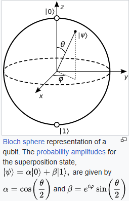 Remember that global phase is not visualized in the bloch sphere.
#### (Set of) Stabilizers (Mostly used in Quantum Error Correction):
* Stabilizer is a speical gate that doesn't change the state. E.g.
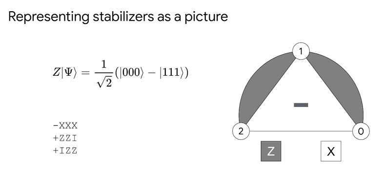
- e.g $\ket{\Psi} = \frac{1}{\sqrt{2}}(\ket{000}+\ket{111})$ is stablilized by three independent stabilizers: $+XXX$, $+ZZI$, $IZZ$,
- And we can use $\{+XXX, +ZZI, IZZ\}$ to represent the state.
- Notice that set $\{+XXX, +ZZI, IZZ, ZIZ\}$ is not a set of stablizer because $ZIZ=(ZZI)(IZZ)$.
* Vis:
- 
### Operations:
#### Gates:
* Engineer PoV: a function that map one (or more) state into another (other states).
* Math:
* $U\ket{\psi} = \ket{\phi}$, where $U$ is a Unitary matrix ( $U^{\dagger}U=I$, length unchanged after transformation) because both $\ket{\psi}$ and $\ket{\phi}$ are valid states.
* Common Single Qubit Gates:
| Gate Symbol | Name | Common Usage | Matrix | $U\ket{0}\space$ | $U\ket{1}$ | $U\ket{+}$ | $U\ket{-}$ | Eigenvalues | Eigenstates |
| :--: | :--: | :--- | :--: | :--: | :--: | :--: | :--: | :--: | :--: |
| **X** | Pauli-X (NOT) | Bit-flip | $$\begin{bmatrix} 0 & 1 \\ 1 & 0 \end{bmatrix}$$|$$\ket{1}$$|$$\ket{0}$$|$$\ket{+}$$|$$-\ket{-}$$|$$+1, -1$$|$$\ket{+}, \ket{-}$$ |
| **Z** | Pauli-Z (Phase) | Phase-flip; adds a relative phase of $\pi$ ( $e^{i\pi} = -1$ ) to the $\ket{1}$ component. | $$\begin{bmatrix} 1 & 0 \\ 0 & -1 \end{bmatrix}$$|$$\ket{0}$$|$$-\ket{1}$$|$$\ket{-}$$|$$\ket{+}$$|$$+1, -1$$|$$\ket{0}, \ket{1}$$ |
| **H** | Hadamard | Creates superposition; changes basis from Z (computational) to X (superposition). | $$\frac{1}{\sqrt{2}}\begin{bmatrix} 1 & 1 \\ 1 & -1 \end{bmatrix}$$|$$\ket{+}$$|$$\ket{-}$$|$$\ket{0}$$|$$\ket{1}$$|$$+1, -1$$|$$\cos\frac{\pi}{8}\ket{0} + \sin\frac{\pi}{8}\ket{1},$$ $$\sin\frac{\pi}{8}\ket{0} - \cos\frac{\pi}{8}\ket{1}$$ |
| **Y** | Pauli-Y | Bit-flip and Phase-flip combined (with a global phase of $i$ ). | $$\begin{bmatrix} 0 & -i \\ i & 0 \end{bmatrix}$$|$$i\ket{1}$$|$$-i\ket{0}$$|$$-i\ket{-}$$|$$i\ket{+}$$|$$+1, -1$$|$$\frac{\ket{0} + i\ket{1}}{\sqrt{2}} (\ket{i}),$$ $$\frac{\ket{0} - i\ket{1}}{\sqrt{2}} (\ket{-i})$$ |
| **S** | Phase (S) | Adds a relative phase of $\frac{\pi}{2}$ ( $e^{i\pi/2} = i$ ) to the $\ket{1}$ component. Often called $\sqrt{Z}$. | $$\begin{bmatrix} 1 & 0 \\ 0 & i \end{bmatrix}$$|$$\ket{0}$$|$$i\ket{1}$$|$$\frac{\ket{0} + i\ket{1}}{\sqrt{2}}$$|$$\frac{\ket{0} - i\ket{1}}{\sqrt{2}}$$|$$1, i$$|$$\ket{0}, \ket{1}$$ |
* Multi-Qubit Gates
* Control gates: only apply to the target qubit when the controlled qubit is $\ket{1}$
* CNOT (CX)
* C-Z
<style>
th, td {
border: 1px solid gray; /* Sets a 1px solid black border for the table and all cells */
padding-left: 0.4em;
padding-right: 0.4em;
}
</style>
* Schrodinger Equation:
* Schrodinger Equation: $$\hat{H} \Psi(\mathbf{r}, t) = i\hbar \frac{\partial}{\partial t} \Psi(\mathbf{r}, t)$$ where
* $\Psi(\mathbf{r}, t)$: Wave Function that contains the information of system at position $\mathbf{r}$ and time $t$
* $\hat{H}$: Hamiltonian Operator, representing the energy of the system
* $\hbar$: Reduced Planck Constant
* It describes the relationship between energy and system change.
* It can be simplied as $$\hat{H} \Psi(t) = i\hbar \frac{\partial}{\partial t} \Psi(t)$$ in QC
* We don't care about the position of that qubit too much in algorithm.
* It's critical in Q'chemical or Q'material.
* $\Psi(\mathbf{r}, t)$ is the complete wave function while $\ket{\Psi(t)}$ can be simplified as a vector.
* Relationship with Quantum gate:
* The solution is: $$\Psi(t) = e^{-i \hat{H} t / \hbar}\Psi(0) = U(t) \Psi(0)$$
* This means with energy $\hat{H}$ for $t$ time, we can transform $\Psi(0)$ into $ e^{-i \hat{H} t / \hbar}\Psi(0) $
* If we control the $\hat{H}$ and $t$ precisely so that $e^{-i \hat{H} t / \hbar} = \frac{1}{\sqrt{2}}\begin{pmatrix} 1 & 1 \\ 1 & -1 \end{pmatrix}$ then we build a $H$ gate.
* If we apply that $\hat{H}$ with $2t$ time (double the duration), then the gates becomes $U=H\cdot H = I$. If the original $\hat{H}$ is mapped to $S$ gate, then we get $U=S\cdot S=Z$ gate.
* What if the machine apply $1.0005t$ time? Then we need QEC algorithm to calibrate (not correction the original qubit!) at the decoding time.
* other anti-error algorithm? VQE (need more research).
#### Measurement
* Measurement will collapse the system into one possible state. The probability is the coefficient (sqr) term of that state in the expression.
* Regular measurement gives $\ket{0}$ or $\ket{1}$ result.
* Measure can be visualized as a gate M (althought it's not).
* $M_x$ is a special measure on the X-axis and gives $\ket{+}$ or $\ket{-}$. Can be achieved by circuit `-H-M`.
#### Annealing
Quantum Simulated Annealing is totally different way to build a quantum system than gated-based circuit. It uses Adiabatic Evolution:
$$i\hbar \frac{\partial}{\partial t} |\Psi(t)\rangle = H(t) |\Psi(t)\rangle$$
where $$H(t) = A(t) H_{init} + B(t) H_{problem}$$
* $H_{init}$ is the Transverse Field (initial states, like $\ket{+}$ for all qubits).
* $H_{problem}$ the hamiliton of the problem. Usualy Ising model
* e.g. $H(\mathbf{x}, \mathbf{y}) = - \sum v_i x_i + \lambda \left( \sum w_i x_i + \sum_{j=0}^{k} 2^j y_j - W \right)^2$ in Knapsack question.
* When $t$ increases, $A(t)$ decreases and $B(t)$ increases.
QSA builts the final target for the problem and gradually shift the qubit to the global minial using the Quantum tunneling effects. It's totally different from the gate-based circuit and won't be dicussed in general QC algorithm design.
### Tricks:
These are some "tricks" that I found intriguing and important when learning multiple quantum algorithms. Each of them is actually a combination of regular gates but arranged in a delicated way, which can be applied in multiple questions. Like "binary-search" in classic algorithms, its methodology is used in element searching, answer bisecting, data structure design etc.
#### Superposition
* Definition:
* Where a qubit is not on $\ket{0}$ or $\ket{1}$ state.
* It can collapse into either 0 or 1 when measured.
* When operated, both 0 and 1 cases are explored (in parallel universe?)! That's mainly why $n$ quantum qubits are $2^n$ more powerful than $n$ classic bits.
* Example procedure:
* Apply `-H-` gate to $\ket{0}$ to get a superposition $\ket{+}$
* Usage:
* Almost in all QC algorithms. To explore all posibilities in a quick way.
#### Entanglement
* Definition:
* Multiple qubits are linked in a system where measurement of anyone of the qubits might change the result probability of the rest of the system.
* e.g. $\ket{q_1q_0} = \sqrt{0.3}\ket{00}+\sqrt{0.7}\ket{11}$
* When measure individually and only once, both $\ket{q_1}$ and $\ket{q_0}$ has $70\%$ to collapse to $1$.
* After measuring $q_1$, if we got $0$, then measurement of $q_0$ must be $0$ because the system collapses to $\ket{00}$ state.
* Example procedure:
* Apply `H` to $\ket{q_0}$ and then `CNOT(q_0, Q_1)` will create a Bell's state $\ket{\Phi ^{+}} = \frac{1}{\sqrt{2}}(\ket{00}+\ket{11}) $
* Most multi-qubit gate will introduce entanglement.
* Usage:
* In most QC algorithms. Information of different qubits are carried together through the entanglement.
* QEC, Quantum teleportation.
#### Partial measurement
* Definition:
* Only measuring a partial set of qubits in an entangled system while keep other qubits still in its superposition.
* e.g. in system $\ket{q_1q_0} = \sqrt{0.2}\ket{00}+\sqrt{0.4}\ket{10}+\sqrt{0.4}\ket{11}$
* if we only measure $q_1$ and get result $1$, then we know the system collapses into $\ket{q_1q_0} = \sqrt{0.5}\ket{10}+\sqrt{0.5}\ket{11} = \ket{1}\ket{+}$
* Procedure:
* Just measure subset of the entangled qubits.
* Usage:
* e.g. In Quantum teleportation, we partially measure 2 qubits in a 3 qubits system and use the results to adjust the untouched qubit.
* (unverified) For some cases, use the partial measurement to scope down the candidate states.
#### Oracle
* Definition:
* Sometimes we need to calculate the function value $f$ given input $\ket{x}$. However, such $F$ ( $F\ket{x}=\ket{f(x)}$ ) might not impossible to build in the quantum world (not a unitary matrix).
* Logical gates like $AND(bit_0, bit_1)$ or $OR(bit_0, bit_1)$ are invalid quantum gates.
* Procedure:
* Instead, we need to use an ancilla qubit to carry the output: $$\begin{align*}U(\ket{x}\ket{0}) &= \ket{x}\ket{f(x)} \\ U(\ket{x}\ket{1}) &= \ket{x}\ket{1\oplus f(x)}\end{align*}$$, such $F$ oracle can be a valid quantum gates.
* Advanced:
* Apply `X-H` gate the ancilla qubit first and we will get: $$\begin{align*} U(\ket{x}H(X(\ket{0}))) &= U(\ket{x}H(\ket{1})) \\ &= U(\ket{x}\ket{-}) \\ &= U(\ket{x}\ket{0}) - U(\ket{x}\ket{1}) \\ &= U(\ket{x}\ket{f(x)}) - U(\ket{x}\ket{1\oplus f(x)}) \\ &= \begin{cases} \ket{x}\ket{0} - \ket{x}\ket{1} = \ket{x}\ket{-} & \text{when } f(x)=0 \\ \ket{x}\ket{1}-\ket{x}\ket{0} = -\ket{x}\ket{-} & \text{when } f(x)=1 \end{cases} \\ &= (-1)^{f(x)}\ket{x-} \end{align*}$$
* This is useful in some problems when we want to treat $x$ different based on $f(x)$
* Usage:
* When a (black-box) function is given. You can wrap any expensive procedure (not only in quantum world) as a function and use the Oracle trick.
* The idea of ancilla qubit can be applied to any discrete function/non-unitary transformation.
#### Phase kickback
* Definition:
* When applying a control U gate to a target qubit, if the target is $U$ 's eigenstate $\ket{u}$ (i.e. $U\ket{u}=lambda\ket{u}$ ), then the target qubit will be unchanged but the eigenvalue $\lambda$ will be "kicked back" to the control qubit: $$\begin{align*} CU((\alpha\ket{0}+\beta\ket{1})\ket{u}) &= CU(\alpha\ket{0}\ket{u})+CU(\beta\ket{1}\ket{u}) \\ &= \alpha\ket{0}\ket{u}+\beta\ket{1}U(\ket{u}) \\ &= \alpha\ket{0}\ket{u}+\textcolor{red}{\lambda}\beta\ket{1}\ket{u} \\ &= (\alpha\ket{0}+\textcolor{red}{\lambda}\beta\ket{1})\ket{u} \end{align*} $$
* Sometime we use eigenphase $\phi$ instead ( $\lambda = e^{i\phi}$ )
* Procedure:
* Use when target states is in a special eigenstate. Prepare the detect qubit as control qubit, apply C-U Gate, and process the result of detect qubit.
* Usage:
* When we want to "poke" the target qubit (using the probe qubit as controlled bit) but don't want to impact it.
* Comment: My favorite trick
* advanced:
* What if target qubit is not in eigenstate?
* Let's assume there are two eigenstates: $U|u_1\rangle = e^{i\phi_1}|u_1\rangle$, $U|u_2\rangle = e^{i\phi_2}|u_2\rangle$
* And $|\psi_{target}\rangle = c_1|u_1\rangle + c_2|u_2\rangle$
* When we set the control qubit to $\ket{+}$, we will get:
$$|\Psi_{final}\rangle = c_1 \underbrace{\left( \frac{|0\rangle + e^{i\phi_1}|1\rangle}{\sqrt{2}} \right)}_{\text{Kickback } \phi_1} \otimes |u_1\rangle + c_2 \underbrace{\left( \frac{|0\rangle + e^{i\phi_2}|1\rangle}{\sqrt{2}} \right)}_{\text{Kickback } \phi_2} \otimes |u_2\rangle$$
### Intro Problmes/Algorithms:
TBA